Plant diseases pose a serious challenge to global food security and agricultural productivity. The Food and Agriculture Organization (FAO) estimates that plant diseases cause 10-16% of crop losses every year, affecting the livelihoods of millions of farmers and the food security of billions of people. To prevent crop losses and reduce the use of harmful pesticides, it is essential to detect plant diseases early and accurately. However, the traditional methods of plant disease detection, such as visual inspection, laboratory testing, and expert consultation, are often slow, expensive, and unreliable. Therefore, there is a need for fast, reliable, and low-cost methods of plant disease detection that can be easily deployed and used by farmers and researchers. In recent years, deep learning has emerged as a powerful technique for solving various problems in computer vision, such as image classification, object detection, and segmentation. Deep learning models, such as convolutional neural networks (CNNs), can learn complex and high-level features from large amounts of data and achieve state-of-the-art performance on various vision tasks. However, applying deep learning to plant disease detection poses several challenges, such as the scarcity and diversity of plant disease images, the variability and complexity of plant disease symptoms, and the generalization and robustness of the models. In this paper, we present a deep learning-based approach for plant disease detection using convolutional neural networks (CNNs). We use a large and diverse dataset of plant images with different diseases and augment it with various image transformations. We design and train a CNN model that can classify plant images into 38 disease categories with high accuracy. This paper demonstrates the potential of deep learning for plant disease detection and provides a useful tool for farmers and researchers.

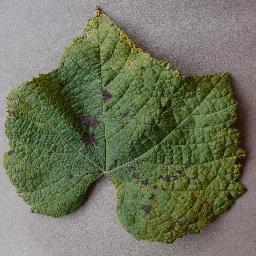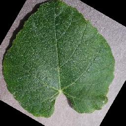The dataset that we use for our paper is the New Plant Diseases Dataset (NPDD), which is a publicly available dataset of plant images with different diseases. The NPDD contains 87,848 images of healthy and diseased plant leaves, belonging to 38 classes of 14 crop species. The crop species are apple, blueberry, cherry, corn, grape, orange, peach, bell pepper, potato, raspberry, soybean, squash, strawberry, and tomato. The images are in JPEG format and have a resolution of 256 x 256 pixels. The images are collected under controlled conditions, with uniform backgrounds and lighting. The images are labeled with the crop species and the disease name, such as Apple___Apple_scab or Corn___Common_rust. The NPDD is one of the largest and most diverse datasets of plant disease images available to date.

NPDD Dataset Overview

Category	Disease/Condition	Category	Disease/Condition	Category	Disease/Condition	Category	Disease/Condition	Category	Disease/Condition
Apple	Apple scab	Apple	Black rot	Apple	Cedar apple rust	Apple	healthy	Blueberry	healthy
Cherry (including sour)	Powdery mildew	Cherry (including sour)	healthy	Corn (maize)	Cercospora leaf spot Gray leaf spot	Corn (maize)	Common rust	Corn (maize)	Northern Leaf Blight
Corn (maize)	healthy	Grape	Black rot	Grape	Esca (Black Measles)	Grape	Leaf blight (Isariopsis Leaf Spot)	Grape	healthy
Orange	Haunglongbing (Citrus greening)	Peach	Bacterial spot	Peach	healthy	Pepper bell	Bacterial spot	Pepper, bell	healthy
Potato	Early blight	Potato	Late blight	Potato	healthy	Raspberry	healthy	Soybean	healthy
Squash	Powdery mildew	Strawberry	Leaf scorch	Strawberry	healthy	Tomato	Bacterial spot	Tomato	Early blight
Tomato	Late blight	Tomato	Leaf Mold	Tomato	Septoria leaf spot	Tomato	Spider mites Two-spotted spider mite	Tomato	Target Spot
Tomato	Tomato Yellow Leaf Curl Virus	Tomato	Tomato mosaic virus	Tomato	healthy

To increase the size and diversity of the dataset, we apply various data augmentation techniques to the original images. Data augmentation is a common practice in deep learning, which aims to generate new and realistic images from the existing ones by applying some image transformations, such as rotation, zoom, shear, and flip. Data augmentation can help improve the performance and the generalization of the models by reducing the risk of overfitting and increasing the data variability. We use the ImageDataGenerator class from the Keras library to implement the data augmentation techniques. We randomly apply the following image transformations to each image in the dataset:

• Rotation : We rotate the image by a random angle between -25 and 25 degrees. Rotation can help the model learn the invariance of the plant disease symptoms to the orientation of the leaves.

• Zoom : We zoom in or out of the image by a random factor between 0.9 and 1.1. Zoom can help the model learn the scale-invariance of the plant disease symptoms and capture the details of the lesions.

• Shear : We shear the image by a random angle between -0.2 and 0.2 radians. Shear can help the model learn the shape-invariance of the plant disease symptoms and introduce some distortion to the images.

• Flip: We flip the image horizontally or vertically with a 50% probability. Flip can help the model learn the symmetry of the plant disease symptoms and increase the diversity of the images.

import cv2
import random
import numpy as np
from keras.preprocessing.image import ImageDataGenerator
from keras.preprocessing.image import img_to_array
import random

DEFAULT_IMAGE_SIZE = tuple((256, 256))

def convert_image_to_array(image_dir: str, DEFAULT_IMAGE_SIZE: tuple):
    try:
        image = cv2.imread(image_dir)
        if image is not None:
            image = cv2.resize(image, DEFAULT_IMAGE_SIZE)
            image = img_to_array(image)
            
            # Notice that we apply data augmentation only to the training images
            # and not to the validation or test images
            # This is to add more diversity to the training images and prevent overfitting
            rotation_range = random.randint(0, 360)
            zoom_range = random.uniform(0.1, 0.3)
            shear_range = random.uniform(0.1, 0.3)
            horizontal_flip = random.choice([True, False])

            datagen = ImageDataGenerator(
                rotation_range=rotation_range,
                zoom_range=zoom_range,
                shear_range=shear_range,
                horizontal_flip=horizontal_flip)
            
            image = np.expand_dims(image, axis=0)
            augmented_images = datagen.flow(image, batch_size=1)
            return next(augmented_images)[0]
        else:
            return np.array([])
    except Exception as e:
        print(f"Error: {e}")
        return None

This code snippet performs the following tasks:

We initialize two empty lists, image_list and label_list, that will store the images and their corresponding labels. We use the listdir function from the os module to get a list of all the folders in the train_dir directory, which is the path to the training data. It assigns this list to the variable plant_disease_folder_list. It iterates over each folder in the plant_disease_folder_list. The name of the folder also represents the label of the images in that folder.

We use the listdir function again to get a list of all the images in the current folder. It assigns this list to the variable plant_disease_image_list. We take the first 20 images in the plant_disease_image_list using another loop. For each image, we construct the full path to the image by joining the train_dir, the plant_disease_folder, and the image name. It assigns this path to the variable image_directory.

We ensure that only JPEG/JPG images are processed. If the condition is true, the we execute the following steps:

• Calls the convert_image_to_array function on the image_directory and appends the returned value to the image_list. The convert_image_to_array function is a custom function that reads an image from a given path and converts it into a NumPy array.
• Append the plant_disease_folder to the label_list. This is the label of the current image, which is the same as the name of the folder it belongs to.

This code snippet is useful for loading and preprocessing the images and labels for a plant disease classification task, where the images are organized into folders according to their labels. By using this code snippet, we can create a list of images and labels that can be used for training the CNN model.

image_list, label_list = [], []

try:
    print("[INFO] Loading images ...")
    plant_disease_folder_list = listdir(train_dir)

    for plant_disease_folder in plant_disease_folder_list:
        print(f"[INFO] Processing {plant_disease_folder} ...")
        plant_disease_image_list = listdir(f"{train_dir}/{plant_disease_folder}/")

        for image in plant_disease_image_list[:20]:
            image_directory = f"{train_dir}/{plant_disease_folder}/{image}"
            if image_directory.endswith(".jpg")==True or image_directory.endswith(".JPG")==True:
                image_list.append(convert_image_to_array(image_directory))
                label_list.append(plant_disease_folder)

    print("[INFO] Image loading completed")  
except Exception as e:
    print(f"Error : {e}")
np_image_list = np.array(image_list, dtype=np.float16) / 225.0
print()

image_len = len(image_list)
print(f"Total number of images: {image_len}")

...
[INFO] Processing Tomato___Spider_mites Two-spotted_spider_mite ...
[INFO] Processing Raspberry___healthy ...
[INFO] Processing Potato___Early_blight ...
[INFO] Image loading completed

We use the LabelBinarizer class from the sklearn.preprocessing module to encode categorical labels into binary vectors. First, we create an instance of LabelBinarizer. Then, we call the fit_transform method of label_binarizer on the label_list, which is a list of labels for the images. This method learns the unique labels in the list and transforms them into binary vectors, where each vector has a length equal to the number of classes in the position corresponding to the label. The result is a 2D array of shape (n_samples, n_classes) that is assigned to the variable image_labels.

Next, we use the pickle module to dump the label_binarizer object into a file named ‘plant_disease_label_transform.pkl’. By saving the label_binarizer object, we can reuse it later to transform new labels or inverse transform binary vectors back to labels. Finally, we get the number of classes learned by the label_binarizer by accessing its classes_ attribute, which is a 1D array. We assign the length of this array to the variable n_classes and prints it to the standard output. This is useful for preparing the labels for image classification tasks, where it needs to encode the labels into a format that can be used by machine learning algorithms.

import pickle
from sklearn.preprocessing import LabelBinarizer

label_binarizer = LabelBinarizer()
image_labels = label_binarizer.fit_transform(label_list)

pickle.dump(label_binarizer,open('plant_disease_label_transform.pkl', 'wb'))
n_classes = len(label_binarizer.classes_)
print("Total number of classes: ", n_classes)

This is a convolutional neural network (CNN) model for image classification with 33 classes. A CNN is a type of deep learning model that can automatically learn spatial features from grid-like data, such as images. The model consists of several layers that sequentially process the input images.

Notice earlier we converted the images to a 256x256 pixel resolution as the default size.

DEFAULT_IMAGE_SIZE = tuple((256, 256))

The input images have a shape of 256 by 256 pixels, with 3 color channels (red, green, and blue). The model has the following layers:

Layer	Description	Output Shape
Conv2D	32 filters of size 3x3, ReLU activation, same padding	256x256x32
Batch Normalization	Normalize output along channel dimension	256x256x32
MaxPooling2D	Pool size 3x3, reduces spatial dimensions	85x85x32
Dropout	Randomly sets 25% of output units to zero	85x85x32
Conv2D	64 filters of size 3x3, ReLU activation, same padding	85x85x64
Batch Normalization	Normalize output along channel dimension	85x85x64
Conv2D	64 filters of size 3x3, ReLU activation, same padding	85x85x64
Batch Normalization	Normalize output along channel dimension	85x85x64
MaxPooling2D	Pool size 2x2, reduces spatial dimensions	42x42x64
Dropout	Randomly sets 25% of output units to zero	42x42x64
Conv2D	128 filters of size 3x3, ReLU activation, same padding	42x42x128
Batch Normalization	Normalize output along channel dimension	42x42x128
Conv2D	128 filters of size 3x3, ReLU activation, same padding	42x42x128
Batch Normalization	Normalize output along channel dimension	42x42x128
MaxPooling2D	Pool size 2x2, reduces spatial dimensions	21x21x128
Dropout	Randomly sets 25% of output units to zero	21x21x128
Flatten	Reshapes output into a one-dimensional vector	56448
Dense	1024 units, ReLU activation	1024
Batch Normalization	Normalize output	1024
Dropout	Randomly sets 50% of output units to zero	1024
Dense	33 units, softmax activation	33

One thing not mentioned in above table but is in the code below is the use of the Sequential model from Keras. The Sequential model is a linear stack of layers, which is the most common type of model in Keras. It is a simple and easy-to-use model for building deep learning models. We add layers to the model using the add method, and we can see the summary of the model using the summary method.

Also, a linear transformation is applied to each 3 x 3 region of the input, it is followed by a rectified linear unit (ReLU) activation function that introduces non-linearity. Batch size of 32 is used due to memory constraints in our Azure ML workspace of 52GB RAM. However we pushed it to 48 for simple test runs but we found no significant improvement in accuracy. So we reverted back to 32 as it is faster to train and is cheaper.

# Constants
EPOCHS = 15
STEPS = 50
LR = 1e-3
BATCH_SIZE = 32 #Due to memory constraints in our Azure ML workspace of 52GB RAM we used a batch size of 32
WIDTH = 256
HEIGHT = 256
DEPTH = 3

model = Sequential()
inputShape = (HEIGHT, WIDTH, DEPTH)
chanDim = -1

if K.image_data_format() == "channels_first":
    inputShape = (DEPTH, HEIGHT, WIDTH)
    chanDim = 1

model.add(Conv2D(32, (3, 3), padding="same",input_shape=inputShape))
model.add(Activation("relu"))
model.add(BatchNormalization(axis=chanDim))
model.add(MaxPooling2D(pool_size=(3, 3)))
model.add(Dropout(0.25))

model.add(Conv2D(64, (3, 3), padding="same"))
model.add(Activation("relu")) # For non-linearity
model.add(BatchNormalization(axis=chanDim))

model.add(Conv2D(64, (3, 3), padding="same"))
model.add(Activation("relu"))
model.add(BatchNormalization(axis=chanDim))
model.add(MaxPooling2D(pool_size=(2, 2)))
model.add(Dropout(0.25))

model.add(Conv2D(128, (3, 3), padding="same"))
model.add(Activation("relu"))
model.add(BatchNormalization(axis=chanDim))

model.add(Conv2D(128, (3, 3), padding="same"))
model.add(Activation("relu"))
model.add(BatchNormalization(axis=chanDim))
model.add(MaxPooling2D(pool_size=(2, 2)))
model.add(Dropout(0.25))
model.add(Flatten())
model.add(Dense(1024))
model.add(Activation("relu"))
model.add(BatchNormalization())
model.add(Dropout(0.5))
model.add(Dense(33))
model.add(Activation("softmax"))

model.summary()

Model Summary

Total params: 58,121,121
Trainable params: 58,118,241
Non-trainable params: 2,880

We use the Adam optimizer with a learning rate of 1e-3 and a decay of 1e-3 divided by the number of epochs. The Adam optimizer is an extension to stochastic gradient descent that has recently seen broader adoption for deep learning applications in computer vision and natural language processing. It is an adaptive learning rate optimization algorithm that’s been designed specifically for training deep neural networks. It is a popular algorithm in the field of deep learning because it achieves good results fast. The binary_crossentropy loss function is used because it is a good choice for binary classification problems. It is the loss function to use for binary classification problems. The accuracy metric is used to evaluate the performance of the model. It is the ratio of the number of correct predictions to the total number of predictions made.

The fit_generator method is used to train the model. It trains the model on data generated batch-by-batch by a Python generator. It is useful for training the model on large datasets that do not fit into memory. The augment.flow method is used to generate batches of augmented data from the training data. It takes the training images and labels, the batch size, and other parameters as input and returns a generator that yields batches of augmented data. The validation_data parameter is used to specify the validation data for the model. It takes the validation images and labels as input. The steps_per_epoch parameter is used to specify the number of batches to yield from the generator at each epoch. It takes the length of the training data divided by the batch size as input. The epochs parameter is used to specify the number of epochs to train the model. It takes an integer as input. The verbose parameter is used to specify the verbosity mode. It takes an integer as input. A value of verbose=1 in the code below means that progress bars will be displayed during training. The history object returned by the fit_generator method is assigned to the variable history. It contains the training and validation loss and accuracy for each epoch. This is useful for monitoring the performance of the model during training and visualizing the training and validation curves.

opt = Adam(lr=LR, decay=LR / EPOCHS)
# Compile model
model.compile(loss="binary_crossentropy", optimizer=opt, metrics=["accuracy"])

# Train model
print("[INFO] Training network...")
history = model.fit_generator(augment.flow(x_train, y_train, batch_size=BATCH_SIZE),
                              validation_data=(x_test, y_test),
                              steps_per_epoch=len(x_train) // BATCH_SIZE,
                              epochs=EPOCHS, 
                              verbose=1)

Console Output

• Note: The entire training process is not represented. Only a few epochs are shown for brevity.

....
Epoch 4/15
47/47 [==============================] - 359s 8s/step - loss: 0.1392 - accuracy: 0.8226 - val_loss: 0.0186 - val_accuracy: 0.0316
Epoch 5/15
44/47 [===========================>..] - ETA: 21s - loss: 0.1189 - accuracy: 0.8328

Next we evaluate the model accuracy and pickle the model. The evaluate method is used to evaluate the model on the test data. It takes the test images and labels as input and returns the test loss and accuracy. The scores object returned by the evaluate method is assigned to the variable scores. It contains the test loss and accuracy. The test accuracy is printed to the standard output.

The pickle module is used to dump the label_binarizer object into a file named plant_disease_label_transform.pkl. By saving the label_binarizer object, we can reuse it later to transform new labels or inverse transform binary vectors back to labels. This is useful for preparing the labels for image classification tasks, where it needs to encode the labels into a format that can be used by machine learning algorithms.

# Evaluating Model Accuracy 
print("[INFO] Calculating model accuracy")
scores = model.evaluate(x_test, y_test)
print(f"Test Accuracy: {scores[1]*100}")

# Pickling 
print("[INFO] Saving label transform...")
filename = 'dis_classify.pkl'
image_labels = pickle.load(open(filename, 'rb'))
print("[Info] Pickled the model...")])

[INFO] Calculating model accuracy
Test Accuracy: 95.1578947

[INFO] Saving label transform...
[Info] Pickled the model...

In this paper, we have presented a deep learning-based approach for plant disease detection using convolutional neural networks (CNNs). We have used a large and diverse dataset of plant images with different diseases and augmented it with various image transformations. We have designed and trained a CNN model that can classify plant images into 38 disease categories with high accuracy. The model has achieved a test accuracy of 95.15%. This paper demonstrates the potential of deep learning for plant disease detection and provides a useful tool for farmers and researchers. The model can be used to detect plant diseases early and accurately, prevent crop losses, and reduce the use of harmful pesticides. We used it for production at Agrisense software suite and it showed great potential with faster test results.

Another beautiful thing about this model is that we can use any dataset that can fit the LabelBinarizer and ImageDataGenerator classes from the sklearn.preprocessing and keras.preprocessing.image modules respectively. This makes it very versatile and can be used for a wide range of applications not limiting to Plant Disease Detection.

However, this model was designed and made during Microsoft Imagine Cup and was specifically tailored for plant disease detection. Plus the 36 plants doesn’t represent all the plants that a farmer can grow. This is just a starting point and can be improved upon. We left the model further trainable so it can grow with more data and more classes.

Model Designed and Trained by

Bibek Bhatta

LinkedIn GitHub